深度学习之图像分类(二)pytorch查看中间层特征矩阵以及卷积核参数
在开始学习深度学习图像分类模型Backbone理论知识之前,先看看如何在 pytorch 框架中查看中间层特征矩阵以及卷积核参数,学习视频源于 Bilibili。
耳听为虚,眼见为实!可视化 feature maps 以及 kernel weights 在论文展示中非常重要,同时对于个人分析神经网络学习的特性也至关重要。本文学习的完整代码详见 此处。
1. 可视化 feature maps
import torch
from alexnet_model import AlexNet
from resnet_model import resnet34
import matplotlib.pyplot as plt
import numpy as np
from PIL import Image
from torchvision import transforms
"""
class AlexNet(nn.Module):
...
def forward(self, x):
# 存储网络中间结果
outputs = []
for name, module in self.features.named_children():
x = module(x)
if name in ["0", "3", "6"]:
outputs.append(x)
# 网络正向传播过程返回的是中间结果
return outputs
"""
# 与训练过程保持一致
data_transform = transforms.Compose(
[transforms.Resize((224, 224)),
transforms.ToTensor(),
transforms.Normalize((0.5, 0.5, 0.5), (0.5, 0.5, 0.5))])
# data_transform = transforms.Compose(
# [transforms.Resize(256),
# transforms.CenterCrop(224),
# transforms.ToTensor(),
# transforms.Normalize([0.485, 0.456, 0.406], [0.229, 0.224, 0.225])])
# create model
model = AlexNet(num_classes=5)
# model = resnet34(num_classes=5)
# load model weights
model_weight_path = "./AlexNet.pth" # "./resNet34.pth"
model.load_state_dict(torch.load(model_weight_path))
print(model)
# load image
img = Image.open("../tulip.jpg")
# [N, C, H, W]
img = data_transform(img)
# expand batch dimension
img = torch.unsqueeze(img, dim=0) # 增加一个 batch 维度
# forward
out_put = model(img)
for feature_map in out_put: # 使用 AlexNet 的话,out_put 是一个 list,有三个元素
# [N, C, H, W] -> [C, H, W]
im = np.squeeze(feature_map.detach().numpy()) # 只输入了一张图,squeeze 压缩掉 batch 维度,detach() 去除梯度信息
# [C, H, W] -> [H, W, C]
im = np.transpose(im, [1, 2, 0])
# show top 12 feature maps
plt.figure()
for i in range(12):
ax = plt.subplot(3, 4, i+1)
# [H, W, C]
# 我们特征矩阵每一个 channel 所对应的是一个二维的特征矩阵,就像灰度图一样,channel = 1
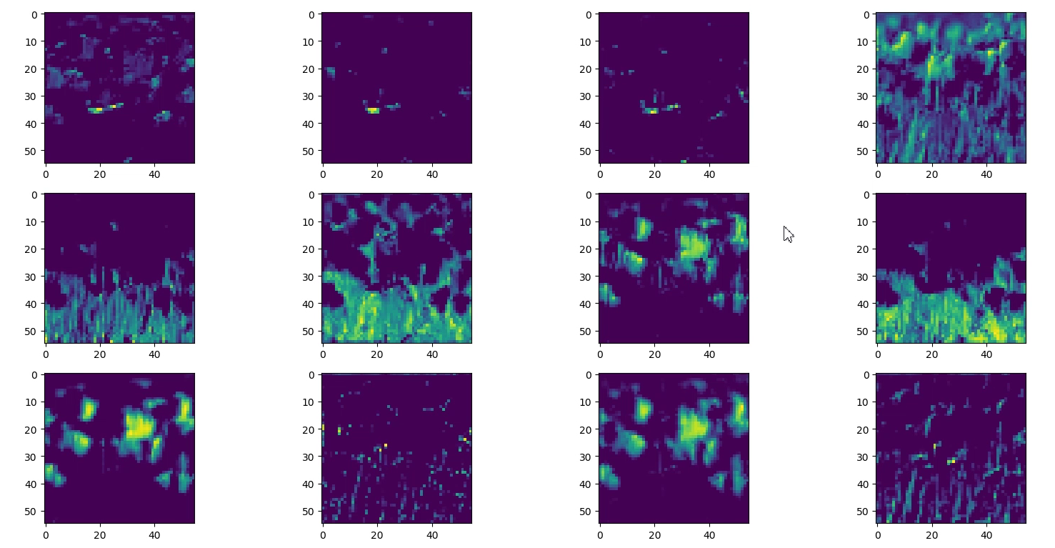
# 如果不指定 cmap='gray' 默认是以蓝色和绿色替换黑色和白色
plt.imshow(im[:, :, i], cmap='gray')
plt.show()
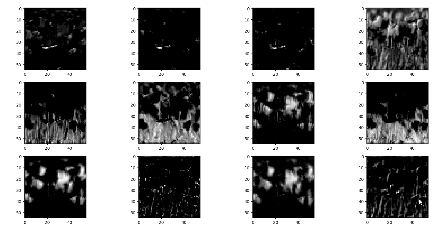
以 AlexNet 为例,下图展示了测试的原始图片:

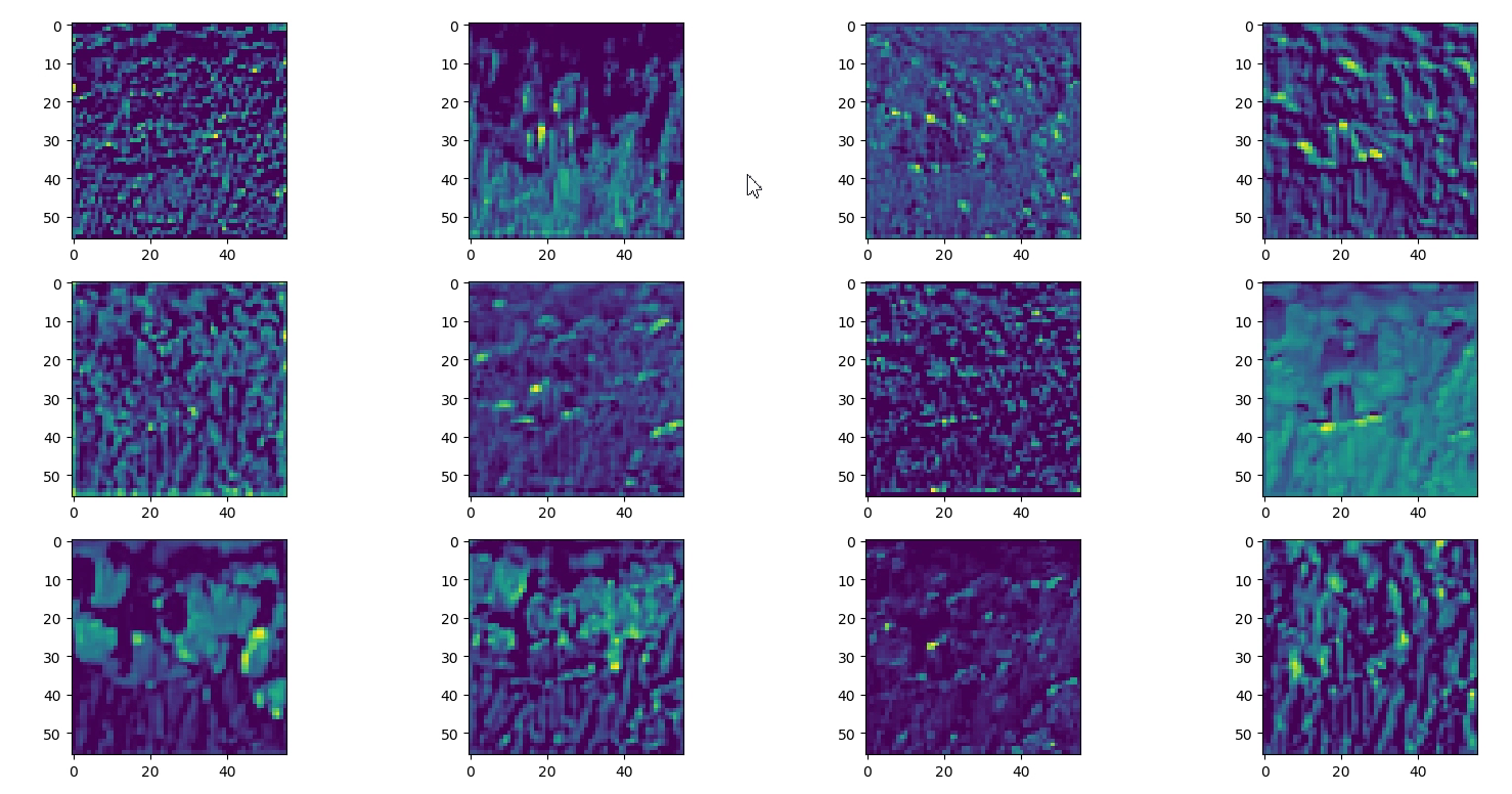
下图打印了第一个卷积层计算得到的前 12 个通道的特征图,每个特征图的切片中可以通过明暗程度来理解卷积层 1 所关注的信息,其中越亮的地方就是卷积核越感兴趣的地方。通过对比原图发现,由于这是卷积层 1 输出的特征矩阵,所以基本还是能看出一些原始图的信息。
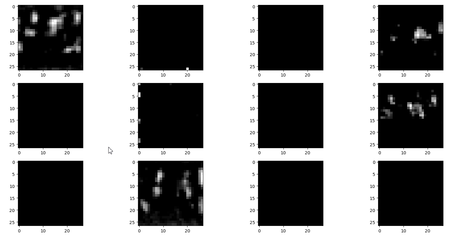
卷积层 2 输出的信息如下所示,由于越往后,抽象程度越高,所以越来越不像所看到的花了。另外有些卷积核没有起到什么作用的,卷积之后得到的特征矩阵都是黑色的,说明根本就没有学到什么有用的信息。
如果之前不增加 cmap='gray' 的话,图片如下所示:
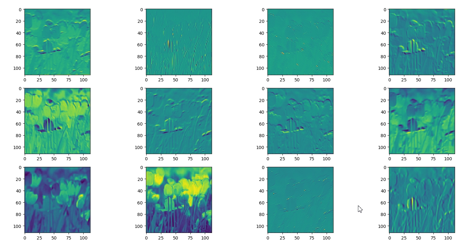
相比而言,使用 ResNet 得到的结果则更好,第一个卷积层输出结果可见它检测到了纹理信息,以及高亮部分展示了花朵等等。ResNet 的 layer 1 输出的特征图结果也比 AlexNet 很多全黑的要好。可能有两个原因造成这种情况,首先是 ResNet 本身比 AlexNet 要好;其次则是 ResNet 使用了迁移学习,用了 ImageNet 预训练的权重来训练的。
哦豁,如果想看全连接层的输出特征矩阵怎么办呢?
2. 可视化 kernel weights
同样以 AlexNet 和 ResNet 为例。
import torch
from alexnet_model import AlexNet
from resnet_model import resnet34
import matplotlib.pyplot as plt
import numpy as np


# create model
model = AlexNet(num_classes=5)
# model = resnet34(num_classes=5)
# load model weights
model_weight_path = "./AlexNet.pth"  # "resNet34.pth"
model.load_state_dict(torch.load(model_weight_path))
print(model)

# model.state_dict() 获取模型所有的可训练参数的字典;.keys() 获取名称
weights_keys = model.state_dict().keys()
for key in weights_keys:
    # remove num_batches_tracked para(in bn)
    if "num_batches_tracked" in key:
        continue

    # [kernel_number, kernel_channel, kernel_height, kernel_width]
    # 输出深度,输入深度,卷积核高,卷积核宽
    weight_t = model.state_dict()[key].numpy()

    # read a kernel information
    # k = weight_t[0, :, :, :]		# 读取第一个卷积核

    # calculate mean, std, min, max
    # 计算均值,标准差,最大值和最小值。
    weight_mean = weight_t.mean()
    weight_std = weight_t.std(ddof=1)
    weight_min = weight_t.min()
    weight_max = weight_t.max()
    print("mean is {}, std is {}, min is {}, max is {}".format(weight_mean,
                                                               weight_std,
                                                               weight_max,
                                                               weight_min))

    # plot hist image
    plt.close()
    weight_vec = np.reshape(weight_t, [-1])		# 卷积核权重展成一维的向量 --- 原始卷积核太小了就3x3
    plt.hist(weight_vec, bins=50)							# 统计卷积核权重值直方图的分布
    plt.title(key)
    plt.show()
下图展示了卷积层 1 的权重以及 bias 的分布。
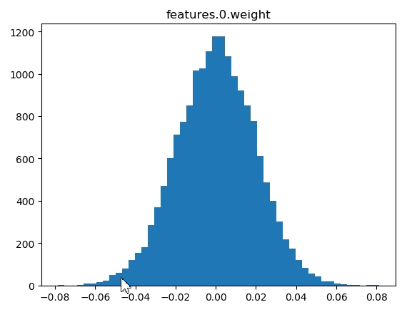
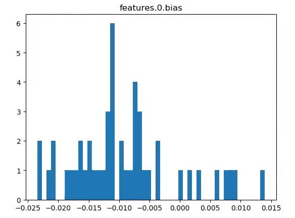
(有时候能看到,很多卷积核参数都是 0…)