深度学习之图像分类(一)分类模型的混淆矩阵
今天开始学习深度学习图像分类模型Backbone理论知识,首先学习分类模型的混淆矩阵,学习视频源于 Bilibili。
1. 混淆矩阵
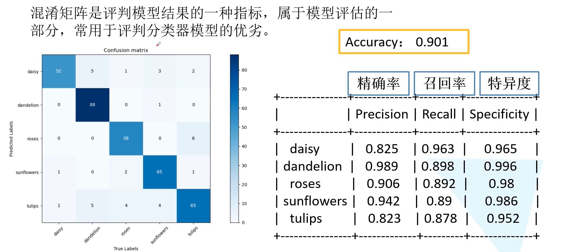
混淆矩阵是评判模型结果的一种指标,属于模型评估的一部分,常用语评判分类模型的优劣。图中左下角为混淆矩阵的一个示例,横坐标为 True Label,纵坐标为 Predicted Label。混淆矩阵每一行对应着预测属于该类的所有样本,混淆矩阵的对角线表示预测正确的样本个数。希望网络预测过程中,将预测类别分布在对角线上。预测值在对角线上分布越密集,则表现模型性能越好。通过混淆矩阵还容易看出模型对于哪些类别容易分类出错。
利用混淆矩阵可以算出精确率,召回率和特异度,这三个指标是对于每个类别得到的结果。注意到,精确率和准确率 Accuracy 是不一样的。准确率是使用所有预测正确样本的个数除以所有样本数量之和。
1.1 二分类混淆矩阵
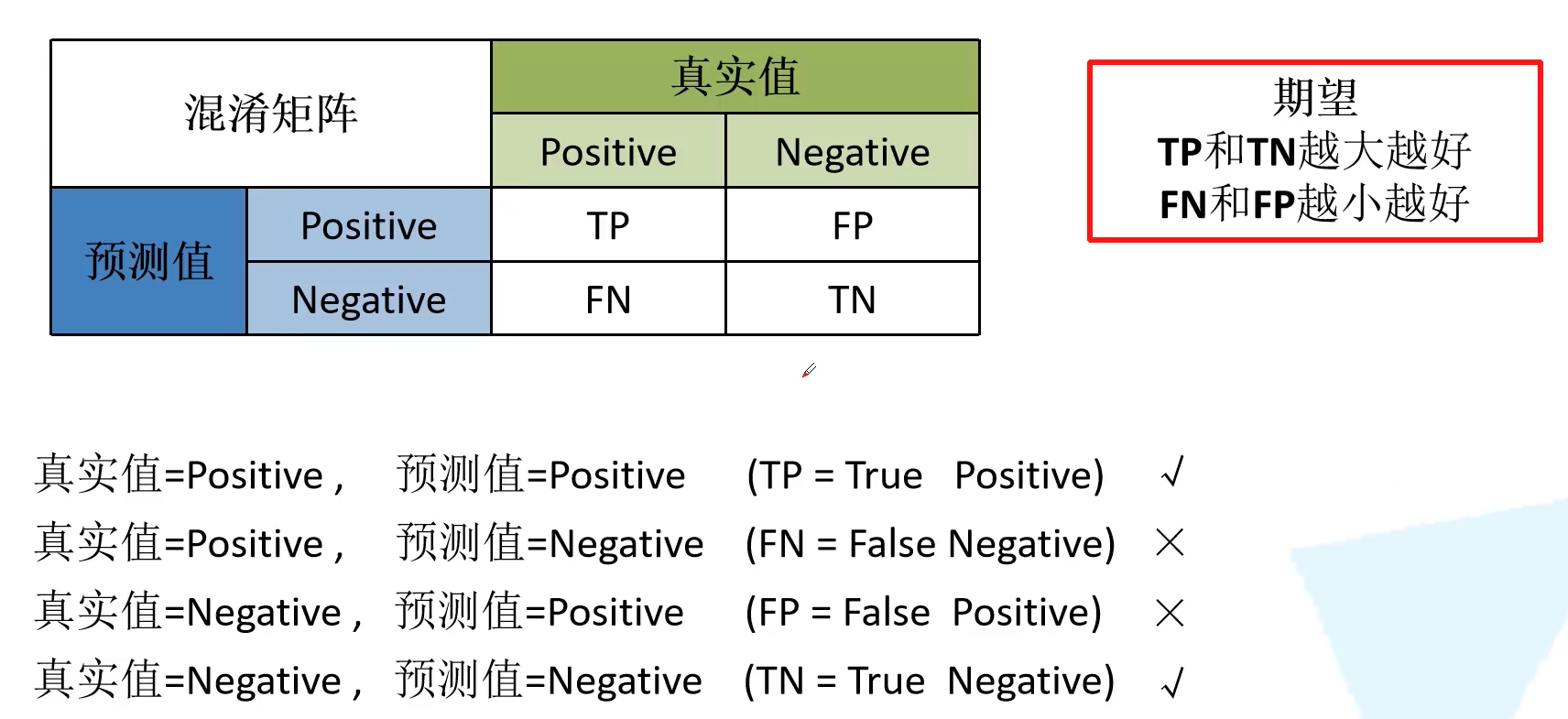
我们首先以二分类混淆矩阵作为讲解。首先每一列表示真实值的标签,每一列表示预测值的标签。Positive 为正样本,Negative 为负样本。此时我们可以有四种分类:
- 真实值为 Positive,预测值为 Positive,标记为 TP
- 真实值为 Positive,预测值为 Negative,标记为 FN — 假阴性
- 真实值为 Negative,预测值为 Positive,标记为 FP — 假阳性
- 真实值为 Negative,预测值为 Negative,标记为 TN
TP 和 TN 都对应着网络预测正确的部分,FP 和 FN 对应着网络预测错误的部分。所以我们期望 TP 和 TN 越大越好,而 FP 和 FN 越小越好。
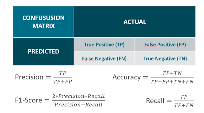
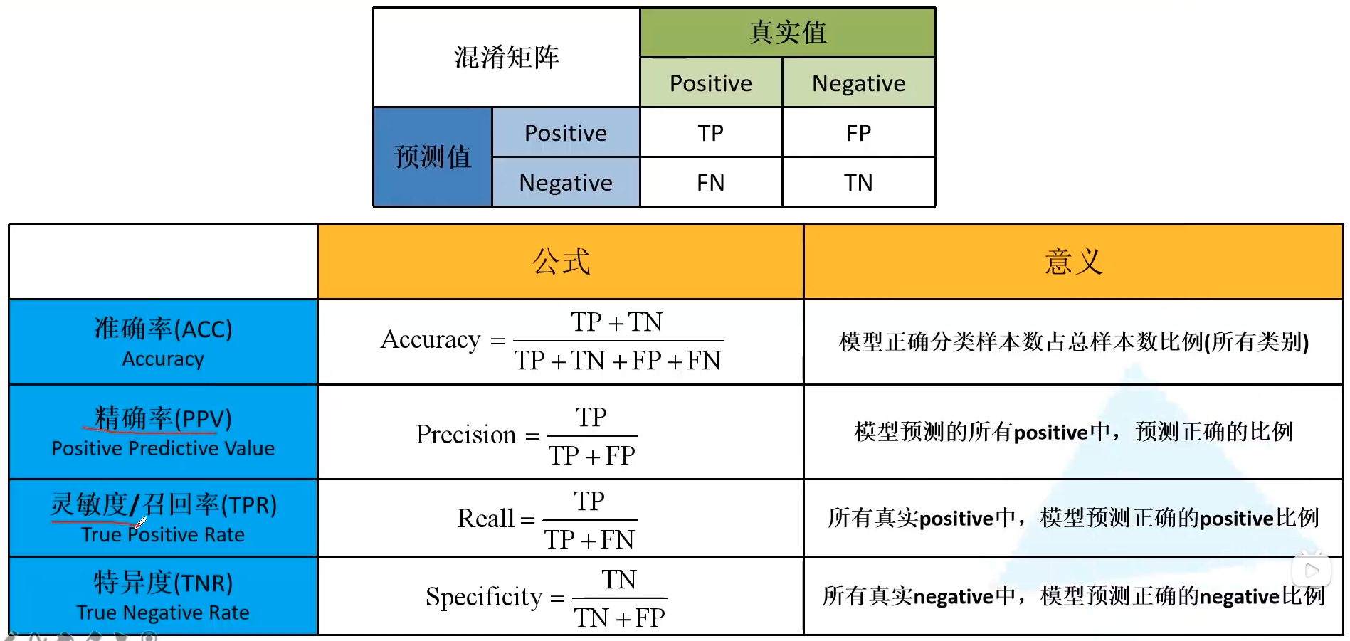
有了 TP、FN、FP、TN 的概念后,我们就可以引入准确率 (Acc, Accuracy)、精确率 (PPV, Positive Predictive Value)、召回率 (TPR, True Positive Rate) 以及特异度 (TNR, True Negative Rate)。注意到,准确率是对所有样本而言的,精确率召回率以及特异度是对于每个类别而言的。计算公式如下表所示:
- 准确率 Acc: 模型正确分类样本数占总样本数的比例(所有类别)
- 精确率 PPV: 模型预测的所有 positive 中,预测正确的比例
- 召回率 TPR: 所有真实 positive 中,模型预测正确的 positive 比例
- 特异度 TNR: 所有真实 negative 中,模型预测正确的 negative 比例
1.2 混淆矩阵计算实例
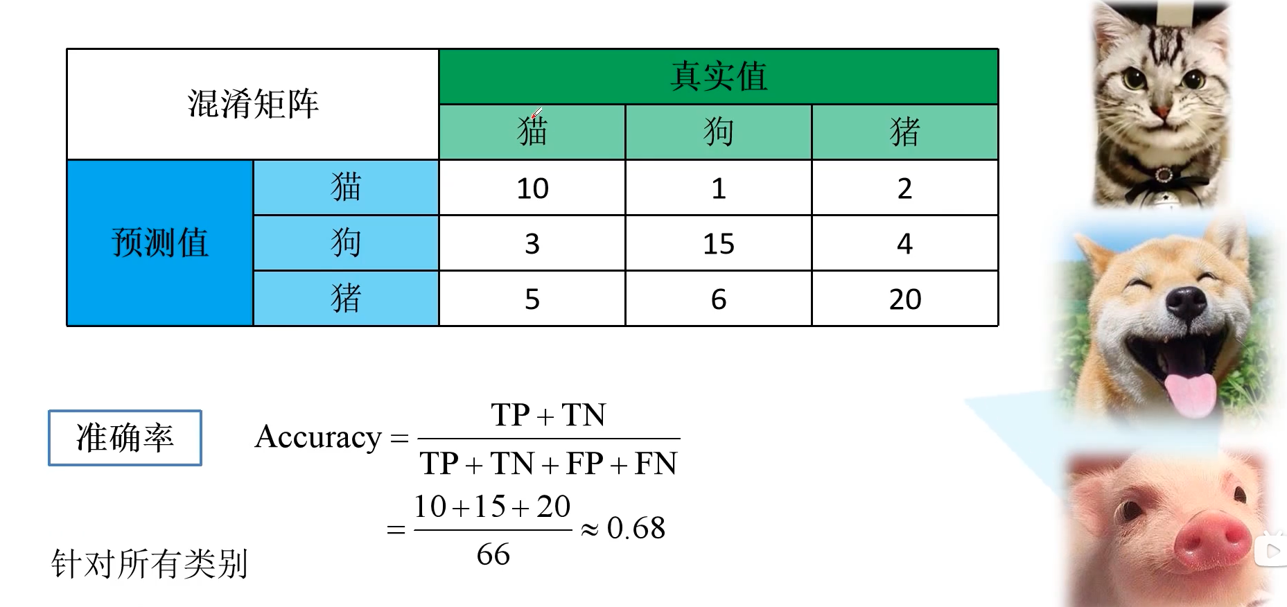
下图给出了一个计算指标的实例,以猫狗猪三分类为例。准确率计算结果如下所示:
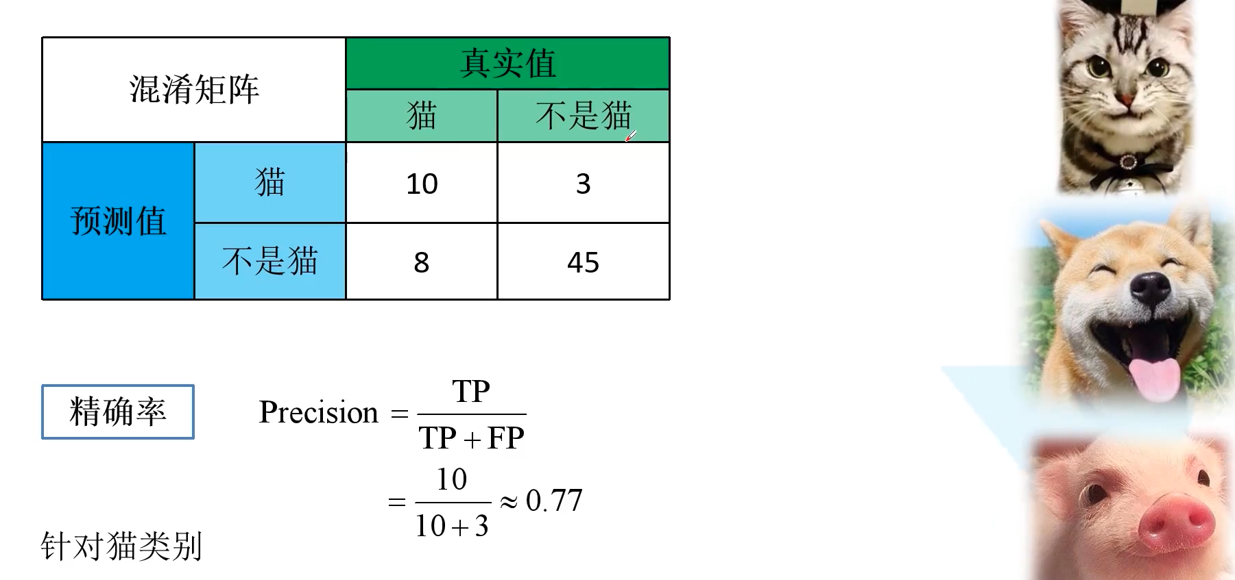
为了算针对 猫 类别的精确率召回率以及特异度,我们统一将狗和猪融合为不为猫的情况。精确率 Precision = 10 / (10 + 3) = 0.77,同样的能算出召回率 Recall = 10 / (10 + 8) = 0.56,特异度 Sepcificity = 45 / (45 + 3) = 0.94。
2. 混淆矩阵代码
完整代码详见 此处。
import os
import json

import torch
from torchvision import transforms, datasets
import numpy as np				# 用 numpy 实现,目的是 pytorch 和 tensorflow 的框架都能使用,label.numpy()
from tqdm import tqdm
import matplotlib.pyplot as plt
from prettytable import PrettyTable

class ConfusionMatrix(object):
    """
    注意,如果显示的图像不全,是matplotlib版本问题
    本例程使用matplotlib-3.2.1(windows and ubuntu)绘制正常
    需要额外安装prettytable库: pip install prettytable
    """
    def __init__(self, num_classes: int, labels: list):
        self.matrix = np.zeros((num_classes, num_classes))	# 初始化混淆矩阵
        self.num_classes = num_classes
        self.labels = labels

    # 混淆矩阵更新
    def update(self, preds, labels):
        for p, t in zip(preds, labels):
            self.matrix[p, t] += 1

    # 计算并打印评价指标
    def summary(self):
        # calculate accuracy
        sum_TP = 0
        for i in range(self.num_classes):
            sum_TP += self.matrix[i, i]				# 对角线元素求和
        acc = sum_TP / np.sum(self.matrix)
        print("the model accuracy is ", acc)

        # precision, recall, specificity
        table = PrettyTable()
        table.field_names = ["", "Precision", "Recall", "Specificity"]	# 第一个元素是类别标签
        for i in range(self.num_classes):			# 针对每个类别进行计算
            # 整合其他行列为不属于该类的情况
            TP = self.matrix[i, i]
            FP = np.sum(self.matrix[i, :]) - TP
            FN = np.sum(self.matrix[:, i]) - TP
            TN = np.sum(self.matrix) - TP - FP - FN
            Precision = round(TP / (TP + FP), 3) if TP + FP != 0 else 0.		# 注意分母为 0 的情况
            Recall = round(TP / (TP + FN), 3) if TP + FN != 0 else 0.
            Specificity = round(TN / (TN + FP), 3) if TN + FP != 0 else 0.
            table.add_row([self.labels[i], Precision, Recall, Specificity])
        print(table)

    # 可视化混淆矩阵
    def plot(self):
        matrix = self.matrix
        print(matrix)
        plt.imshow(matrix, cmap=plt.cm.Blues)		# 从白色到蓝色

        # 设置x轴坐标label
        plt.xticks(range(self.num_classes), self.labels, rotation=45)	# x 轴标签旋转 45 度方便展示
        # 设置y轴坐标label
        plt.yticks(range(self.num_classes), self.labels)
        # 显示colorbar
        plt.colorbar()
        plt.xlabel('True Labels')
        plt.ylabel('Predicted Labels')
        plt.title('Confusion matrix')

        # 在图中标注数量/概率信息
        thresh = matrix.max() / 2
        for x in range(self.num_classes):
            for y in range(self.num_classes):
                # 注意这里的matrix[y, x]不是matrix[x, y]
                # 画图的时候横坐标是x,纵坐标是y
                info = int(matrix[y, x])
                plt.text(x, y, info,
                         verticalalignment='center',
                         horizontalalignment='center',
                         color="white" if info > thresh else "black")
        plt.tight_layout()		# 图形显示更加紧凑
        plt.show()
3. 混淆矩阵用途
- 混淆矩阵能够帮助我们迅速可视化各种类别误分为其它类别的比重,这样能够帮我们调整后续模型,比如一些类别设置权重衰减等
- 在一些论文的实验分析中,可以列出混淆矩阵,行和列均为 label 种类,可以通过该矩阵验证自己 model 预测复杂 label 的能力是否强于其他 model,只要自己 model 将复杂 label 误判为其它类别比其他 model 误判的少,就可以说明自己 model 预测复杂 label 的能力强于其他 model。